Expected Goals Just Don’t Add Up — They Also Multiply.
Exploring Variance in Expected Goals
Soccer and hockey analytical communities have been pleased to discover some measure of shot quality in their sports. While the quantity of shots has been very important in predicting future success, more information from game play-by-plays allows analysts to measure the quality of each shot. We’ve been able to take each shot from a game and assign them a number; these are called “expected goals” (xG for the rest of this article). For example: A shot measured equaling 0.25 xG is determined to be converted into a goal 25% of the time. Many analysts have used seasons of data to populate their models. While they might not agree on the details (“What is a header worth in the EPL?” may differ from model to model; same for the value of a “Shot from the Blue Line in NHL”), overall they agree and have been shown to reliably quantify shot quality. There are a few expected goal models linked at the end of this article if you’re interested in those specifics!
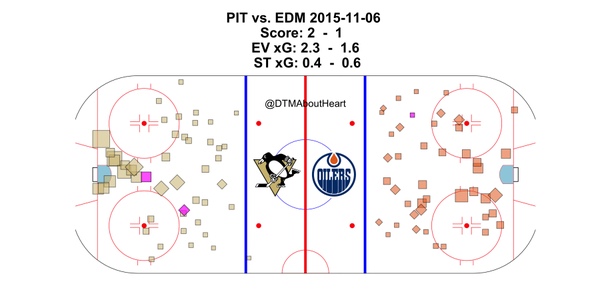
Using this information, we have measured games and seasons in terms of expected goals and can compare to the observed goals. Here are two examples, one in hockey and one in soccer. The Pittsburgh vs Edmonton NHL game ended 2–1; the total xG scoreline would be 2.7–2.2.
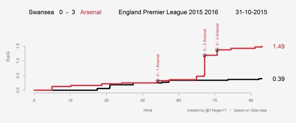
Arsenal won 0–3 with a xG scoreline of 0.39–1.49. In these cases, some may say “The right team won” because the xG and real life scorelines match. However, these values are only adding expected goals. But something is missing. Only adding independent probabilities misses half of the story: variance.
Here’s a simple example to explain what’s missing: Let’s pretend have Team Coin and Team Die. We are going to compare the “number of times the coin lands on heads” to the “number of times the die rolls six”, and compare them like we would a soccer or hockey match.
If you were to flip the coin four times, expected heads would equal 2. But we can observe anything from zero to four heads. Only stating xH = 2 would be leaving out a lot of information! Similarly, if we rolled a six-sided die 12 times, expected sixes would also equal 2. But we could have anywhere from zero to twelve rolls that would result in six.
So if we compared Team Coin vs Team Die, we could get any score from 0–0 to 4–12. Given 4 flips and 12 rolls, the expected scoreline of Team Coin 2–2 Team Die does not accurately portray this possibility space. So how do we better represent the result of Team Coin vs Team Die? We need to measure the variance of these results. Using an expected goals simulator, we can show that in addition to the expected score of 2–2:
- Add Standard Deviation to the scoreline: It would read Coin 2±1 — Die: 2±1.29. The “±1” is the standard deviation of the result. Standard deviation is a number used to tell how measurements for a group are spread out from the average. Team Coin’s score would fall into the spread of ±1 goal 68% of the time and ±2 goals 95% of the time. Die’s “±1.29” denotes that their score will fluctuate more than Coin’s results. (±1.29 68% of the time; ±2.58 95% of the time)
- The Winning Percentage of the two “teams”: Team Coin would win 40% games to Team Die’s 36%, and a draw occurs 24% the time.
- The Points Per Game for each team: Team Coin would earn 1.42 PPG to Team Die’s 1.34 PPG. (This is within the 3-point system; NHL’s 2-point system would require a different calculation.)
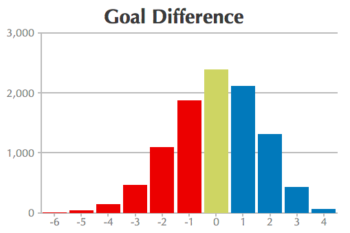
Red: Die — Blue: Coin — Gold: Draw — Y-Axis: Occurrences out of 10,000 sims
In my opinion, Win Percentage would be the most reasonable determination if you’re tweeting out expected goal scores. If you’re including a picture in your report, graphing the goal difference will show the variance in possible results, and allows you to display the probability of each result. In this case, ±0 was the most likely result, followed by +1 Coin, then -1 Die.
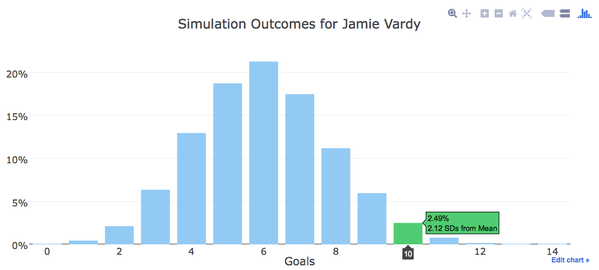
We must also keep this in mind for players. Jamie Vardy is having a heck of a year. 10 goals from 19 shots on target is tough to repeat. Over many simulations, we’d expect 6±1.9 xG from Vardy. This means we would an average of 6 goals from him, and his results would have a Standard Deviation of 1.9 goals.
His observed 10 goals are 2.12 Standard Deviations above the mean, which only happens 2.5% of the time. [10 goals = 6xG + 1.9 SD * 2.12 ] Perhaps the model is missing something that Vardy does well, or more likely, his goalscoring will revert towards his expected average in the rest of the season.
Sustained Attacks
A another instance of expected goals not “adding up” is when you’re evaluating a single attack with multiple shots. Whether that’s a few shots after a zone entry in hockey, or the keeper rebounds the ball and it results in a second shot, adding up expected goals will not give you a clear result. For example:
- Imagine a striker takes a solid shot at the keeper, evaluated at 0.25 xG. It’s deflected by the keeper.
- That midfielder takes a volley, worth 0.4 xG. It bounces off the crossbar.
- The chasing wingback moves into the area, collects the rebound and scores a close header, worth 0.6 xG.
How should we evaluate this attack? If we added these shots together, it would equal 1.25 xG, which is a meaningless number. This would seem to mean that a goal was certain, but we know that’s not true. Likely, but definitely not 100% (or 125%!) certain. If you remember Independent Probabilities from stats class, this will be familiar:
A = 0.25 | A' = 0.75 // P(A) means 25% chance of it happening
B = 0.40 | B' = 0.60 // The ' in B' means not converting the shot.
C = 0.60 | C' = 0.40 // P(Goal) is overall chance of a goal

Addition // Bad
P(Goal) = P(A) + P(B) + P(C) = 0.25 + 0.4 + 0.6 = 1.25

Multiplication // Good
P(Goal) = P(A) + P(A' | B) + P( C | A'| B')
P(Goal) = 0.25 + 0.75*0.40 + 0.60*0.60*0.75
P(Goal) = 0.25 + 0.30 + 0.27
P(Goal) = 0.82
Therefore, we can see that with multiplication, we can appropriately determine the chance of a set of shots producing one goal. In this case, the 3-shot attack would have produced a goal 82% of the time. Edit (2024): This simplified calculation does not incorporate the chance of the rebound turning into another attack, so the 82% number would likely be even lower. Not every shot turns into a rebound into another attack for the offensive team.
If you were to include 1.25 xG in your scoreline instead of 0.82 xG, your expected goals model may overrate teams that created rebounds or unfairly punish teams that give up rebounds. Rebounds are valuable, but must also be evaluated properly, so any expected goals model must keep this in mind. Each model must determine when a shot can be considered independent of any previous attempts on goal. For example: all attacks in a specific zone entry, waiting for a 15 second cool down period after a shot, or waiting for the defense to take control.
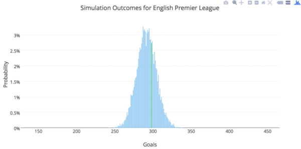
So we’ve covered three very important situations where only showing the sum total of xG doesn’t make the most sense. But at the seasonal level, perhaps it’s not all that bad. We would assume that over time, xG would revert towards the mean. In one such example (973 shots on target), the observed goals of 298 was not far off our expected mean of 290. In a pinch, you would not be far off. However, there may be more variance for an individual team, even over 38/82 games, and quantifying exactly how much a team can vary will require extra research.
Conclusion
Lots of great work has been done in both soccer and hockey to be able to quantify the value of an individual shot. In this article I’ve shown how we can properly combine 2, 3, or 50 shots while accurately portraying all the applicable information. **Summing xG is only half of the story; we must also consider variance as well. **Failure to do so may mislead the reader into taking the wrong conclusion from a simple sum xG scoreline. In the future, we must take the extra step and communicate the entire range of possibilities.
Thanks for reading! If you have any questions or comments, you can contact me on Twitter, and please share if you liked this article!
Addendum
Mark Taylor covered in 2014 how one team can win more when two teams score the same amount of xG. There are even a set of circumstances where you can have a larger sum-total xG, and still lose over time. I’ve left this as an exercise to the reader, and you can use my Match Expected Goals Simulator to discover this scenario.
Expected Goals Models — explanations and twitter handles:
- Michael Caley (@MC_of_A) — Soccer
- American Soccer Analysis (@AnalysisEvolved) — Soccer
- Hockey-Graphs (@DTMAboutHeart & @asmean) — Hockey
- @11tegen11 — Soccer
- Michael Bertin (@bertinbertin) — Soccer
- Paul Riley (@footballfactman) — Soccer
